2.2. Radiometric & Geometric Corrections

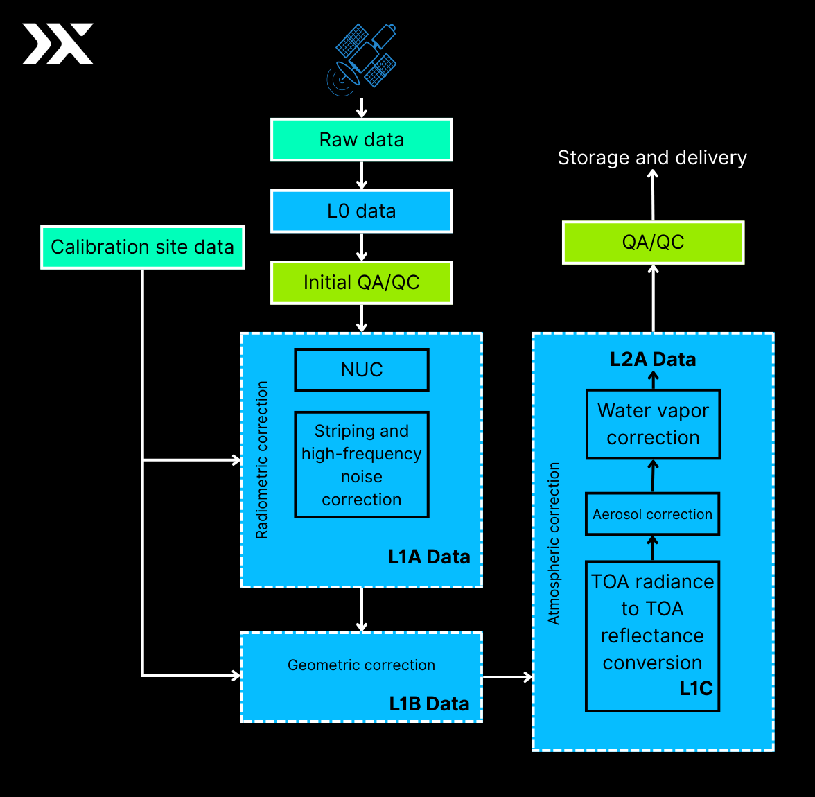
Raw hyperspectral data must be calibrated and corrected to be scientifically meaningful. These corrections convert raw pixel values into accurate surface-level reflectance aligned with real-world coordinates.

Radiometric Calibration (Sensor Level)

Hyperspectral sensors initially record raw data as digital numbers (DNs) corresponding to the intensity of light detected at each wavelength. However, these raw values are not directly usable for material identification or analysis.

Radiometric calibration transforms DNs into at-sensor radiance, a physical measurement of light energy (typically expressed in W·m⁻²·sr⁻¹·µm⁻¹). This step ensures that data from the sensor represents real-world light levels rather than uncorrected instrument responses.

Key elements of radiometric calibration include:

• Non-Uniformity Correction (NUC): Adjusts for differences in sensitivity between individual detector elements.
• Dark Current & Noise Correction: Removes background signal introduced by sensor electronics, thermal effects, or stray light.
• Conversion to Radiance: Applies sensor-specific calibration coefficients (gains, offsets) derived from pre-flight lab calibration.

At this stage, this data is considered Top-of-Atmosphere (TOA) radiance. This data accurately reflects the energy arriving at the sensor, but still includes distortions from the atmosphere and surface conditions.

Geometric Correction & Orthorectification (Scene Level)

To ensure hyperspectral imagery accurately represents real-world locations, geometric corrections must be applied to correct for distortions introduced by terrain, sensor geometry, and platform motion. These corrections enable the hyperspectral data to align precisely with geographic coordinate systems and other spatial datasets.

Key steps:

• Orthorectification: Corrects for terrain-induced distortions by incorporating a Digital Elevation Model (DEM). This ensures that features are represented in their true ground positions, accounting for variations in elevation, sensor tilt, and viewing angle.
• Georeferencing: Aligns the image to a known coordinate system using GPS and Inertial Measurement Unit (IMU) data collected during acquisition, or by using Ground Control Points (GCPs), identifiable features whose precise coordinates are known. This step establishes a spatial reference framework for the dataset.
• Image Registration: Ensures accurate alignment of multiple datasets, such as when comparing hyperspectral images from different dates (multi-temporal analysis) or integrating data from multiple sensors (multi-sensor fusion). Registration minimises spatial offsets between datasets.

Coordinate Systems and Projections

Once georeferenced, hyperspectral data is projected into a standardised map projection to ensure spatial consistency with other geospatial layers. A common projection used in remote sensing is the WGS84 (World Geodetic System 1984), which is the global standard for Earth mapping and GPS systems.

• Projections define how the curved surface of the Earth is translated onto a flat map. Using consistent projections (e.g., WGS84 UTM zones) ensures accurate distance, area, and positional analyses.
• Depending on the region of interest, a Universal Transverse Mercator (UTM) projection based on WGS84 may be used for finer local accuracy.

The result of geometric correction and projection is a geospatially accurate, orthorectified hyperspectral dataset that can be overlaid with other GIS layers (e.g., land cover maps, vector shapefiles) for spatial analysis and visualisation.

Atmospheric Correction Methods (Scene Level)

Hyperspectral data captured by satellite sensors are influenced by the atmosphere. Molecules such as water vapour, carbon dioxide, and ozone, along with aerosols, scatter and absorb incoming solar radiation. These effects distort the raw at-sensor radiance, making it unsuitable for direct quantitative analysis. Atmospheric correction removes these distortions, converting radiance to surface reflectance (a measure of the fraction of incoming light reflected by the surface itself).

A variety of models exist for atmospheric correction:

While these methods are widely used, Pixxel employs a customised, next-generation model, piSOFIT, to achieve high accuracy for its hyperspectral imagery.

Pixxel ISOFIT (piSOFIT) is Pixxel’s customised implementation of NASA JPL’s ISOFIT (Imaging Spectrometer Optimal Fitting) model, designed for precise atmospheric correction of Pixxel’s hyperspectral imagery. piSOFIT simulates how light interacts with the atmosphere and surface, then iteratively adjusts atmospheric and surface parameters to match observed radiance.

Key features:

• Radiative Transfer Modelling – Neural network–accelerated MODTRAN emulator (based on 6S) for fast, accurate simulations.
• Optimal Estimation – Refines aerosol and water vapour estimates using Bayesian priors.
• Uncertainty Quantification – Propagates sensor noise and model variability to produce pixel-level confidence metrics.
• Empirical Line Method – Scene-specific fine-tuning of reflectance retrievals.

Through this process, Pixxel produces two sequential reflectance products:

• L1C (TOA Reflectance): Normalised for solar illumination and geometry.
• L2A (Surface Reflectance): Bottom-of-atmosphere (BOA) imagery corrected for atmospheric scattering, absorption, suitable for quantitative science and operational applications.